Nearest neighbors and vector models – part 2 – algorithms and data structures
This is a blog post rewritten from a presentation at NYC Machine Learning on Sep 17. It covers a library called Annoy that I have built that helps you do nearest neighbor queries in high dimensional spaces. In the first part, I went through some examples of why vector models are useful. In the second part I will be explaining the data structures and algorithms that Annoy uses to do approximate nearest neighbor queries.
Let’s start by going back to our point set. The goal is to find nearest neighbors in this space. Again, I am showing a 2 dimensional point set because computer screens are 2D, but in reality most vector models have much higher dimensionality.
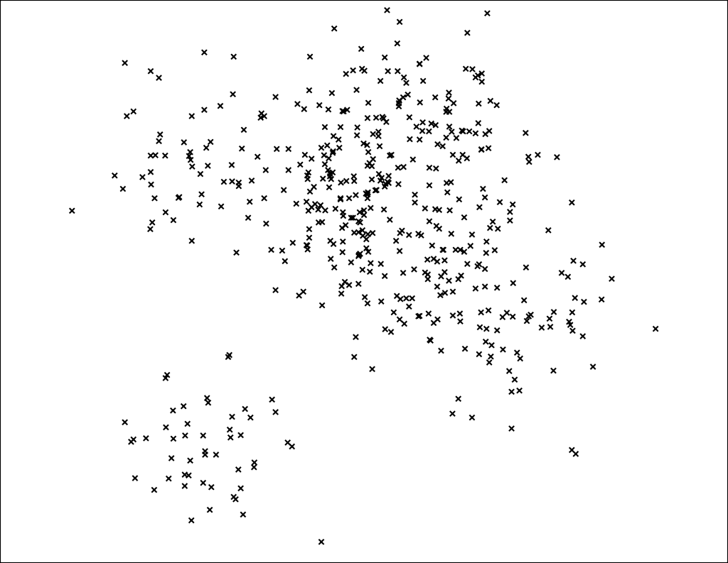
Our goal is to build a data structure that lets us find the nearest points to any query point in sublinear time.
We are going to build a tree that lets us do queries in $$ \mathcal{O}(\log n) $$ . This is how Annoy works. In fact, it’s a binary tree where each node is a random split. Let’s start by splitting the space once:
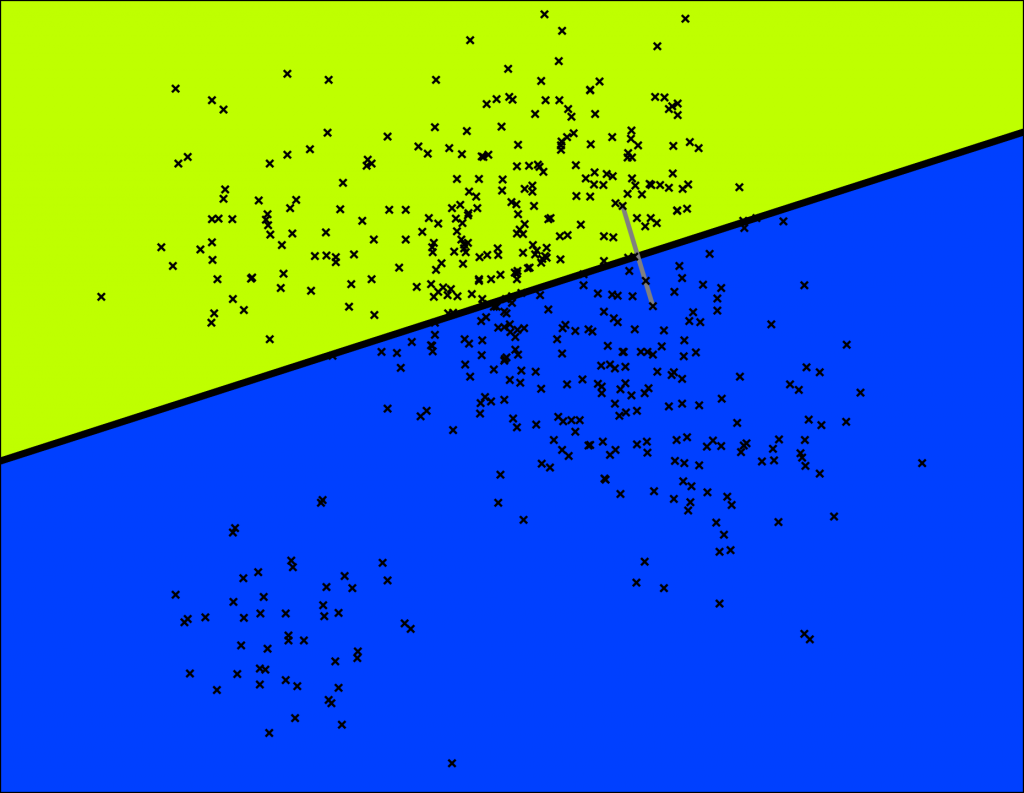
Annoy does this by picking two points randomly and then splitting by the hyperplane equidistant from those two points. The two points are indicated by the gray line and the hyperplane is the thick black line.
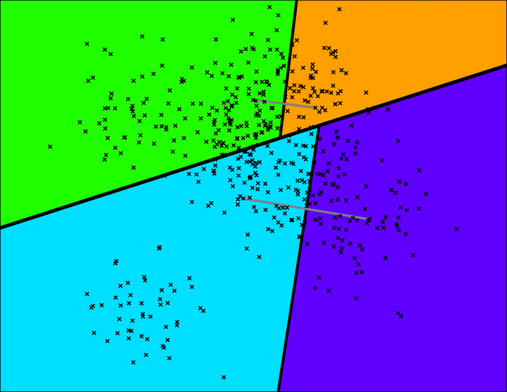
Let’s keep splitting each subspace recursively!
A very tiny binary tree is starting to take shape:
We keep splitting again:
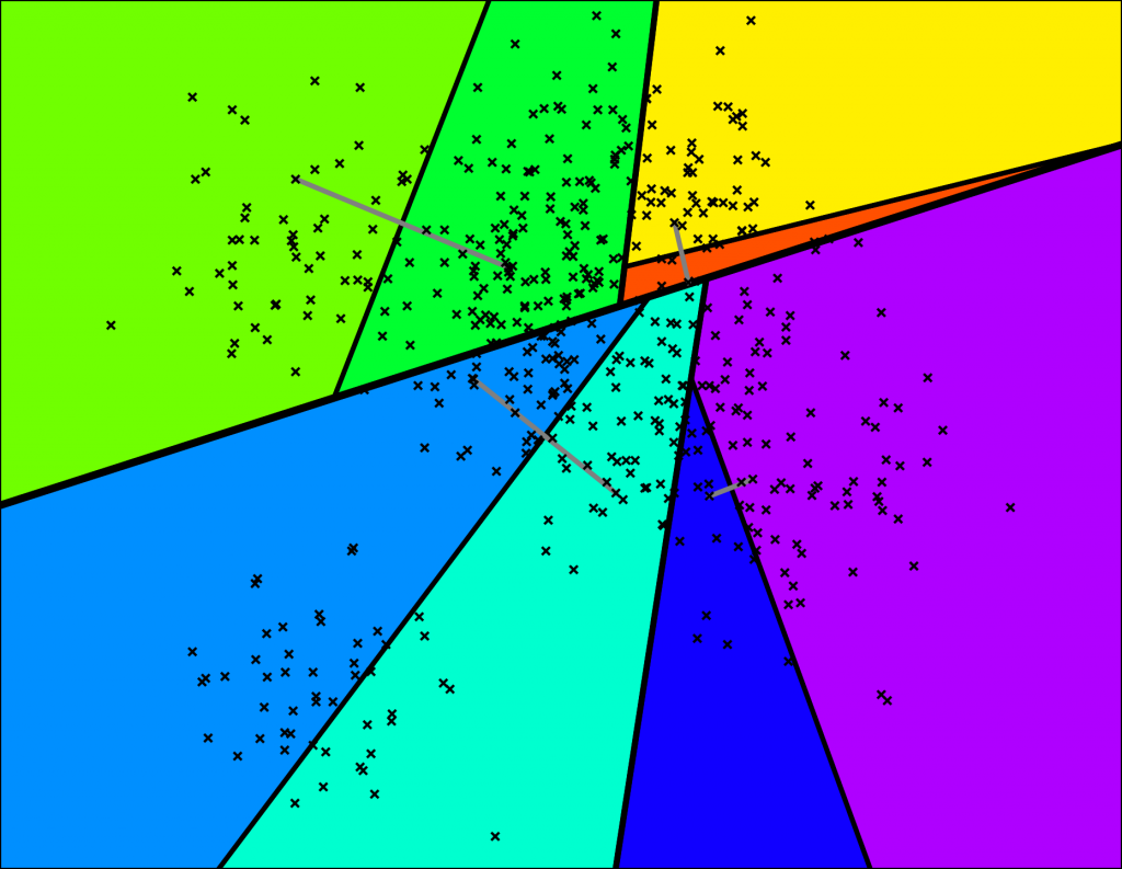
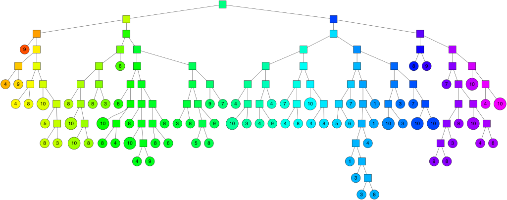
… and so on. We keep doing this until there’s at most K items left in each node. At that point it looks something like this (for K=10):
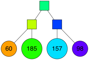
With the corresponding binary tree:
Nice! We end up with a binary tree that partitions the space. The nice thing is that points that are close to each other in the space are more likely to be close to each other in the tree. In other words, if two points are close to each other in the space, it’s unlikely that any hyperplane will cut them apart.
To search for any point in this space, we can traverse the binary tree from the root. Every intermediate node (the small squares in the tree above) defines a hyperplane, so we can figure out what side of the hyperplane we need to go on and that defines if we go down to the left or right child node. Searching for a point can be done in logarithmic time since that is the height of the tree.
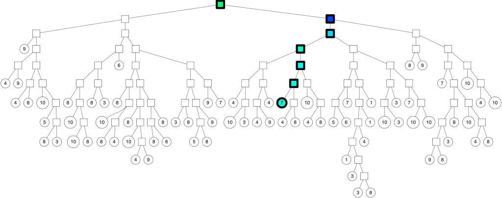
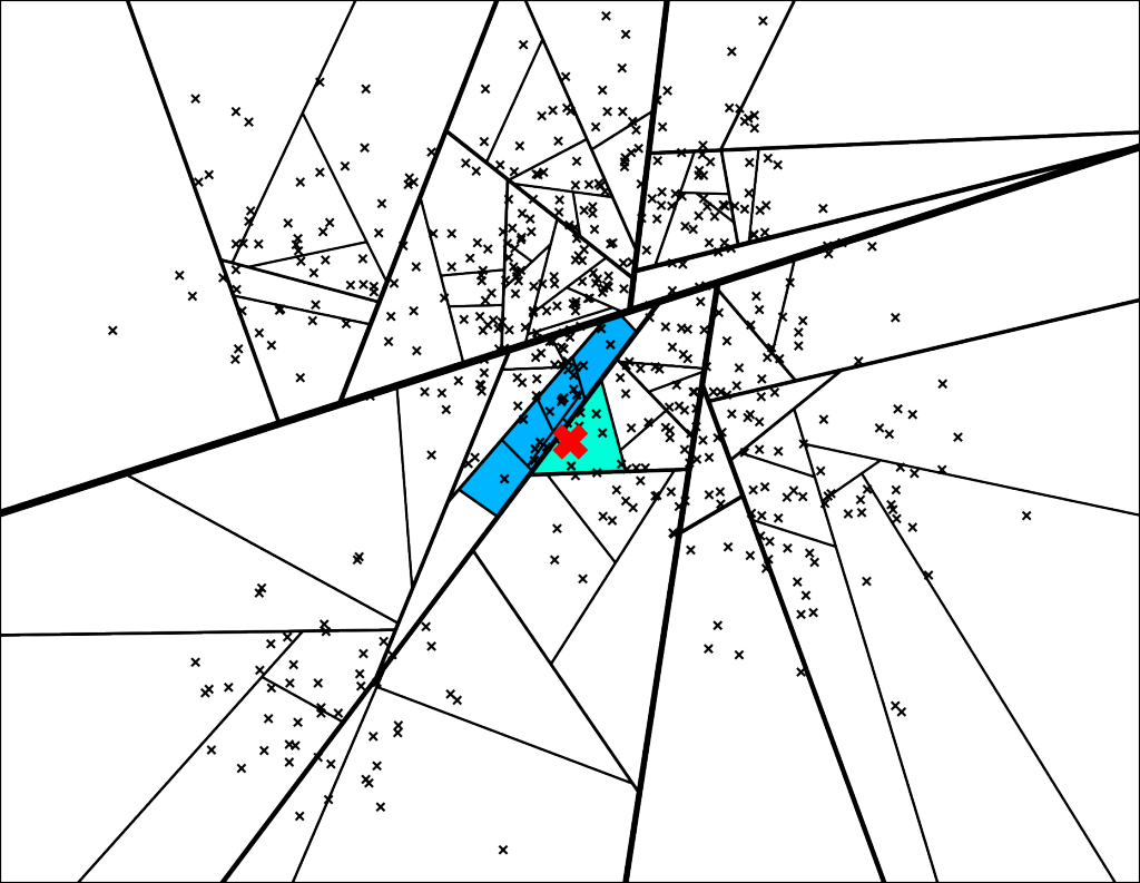
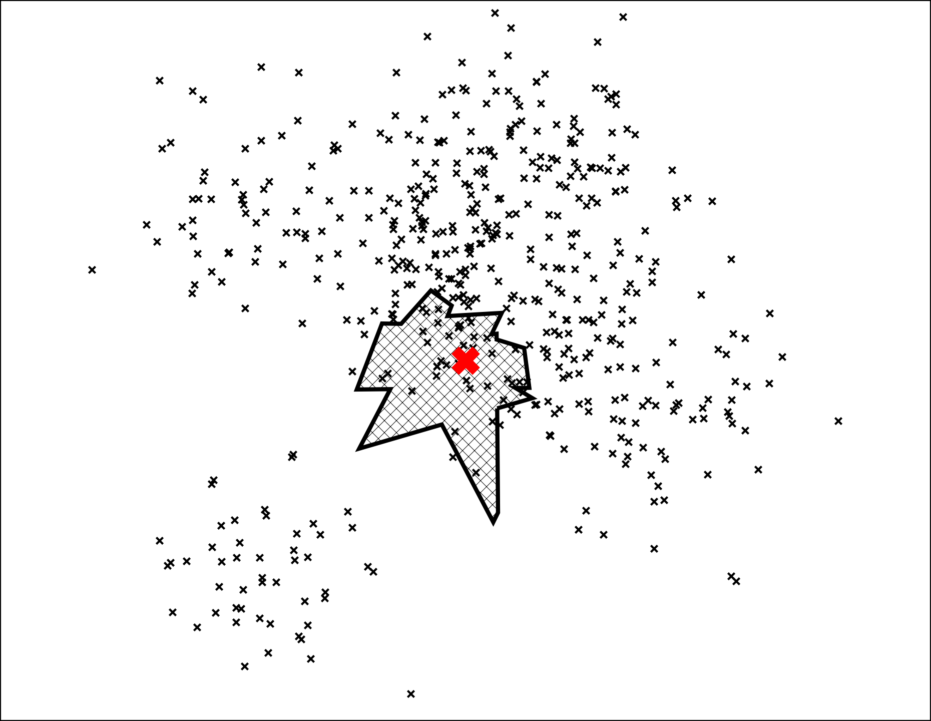
Let’s search for the point denoted by the red X in the plot below:
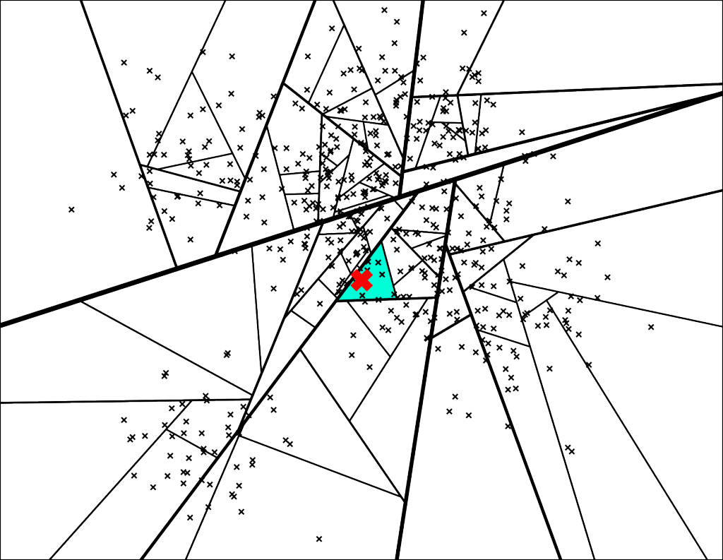
The path down the binary tree looks like this:
We end up with 7 nearest neighbors. Very cool, but this is not great for at least two reasons
- What if we want more than 7 neighbors?
- Some of the nearest neighbors are actually outside of this leaf polygon
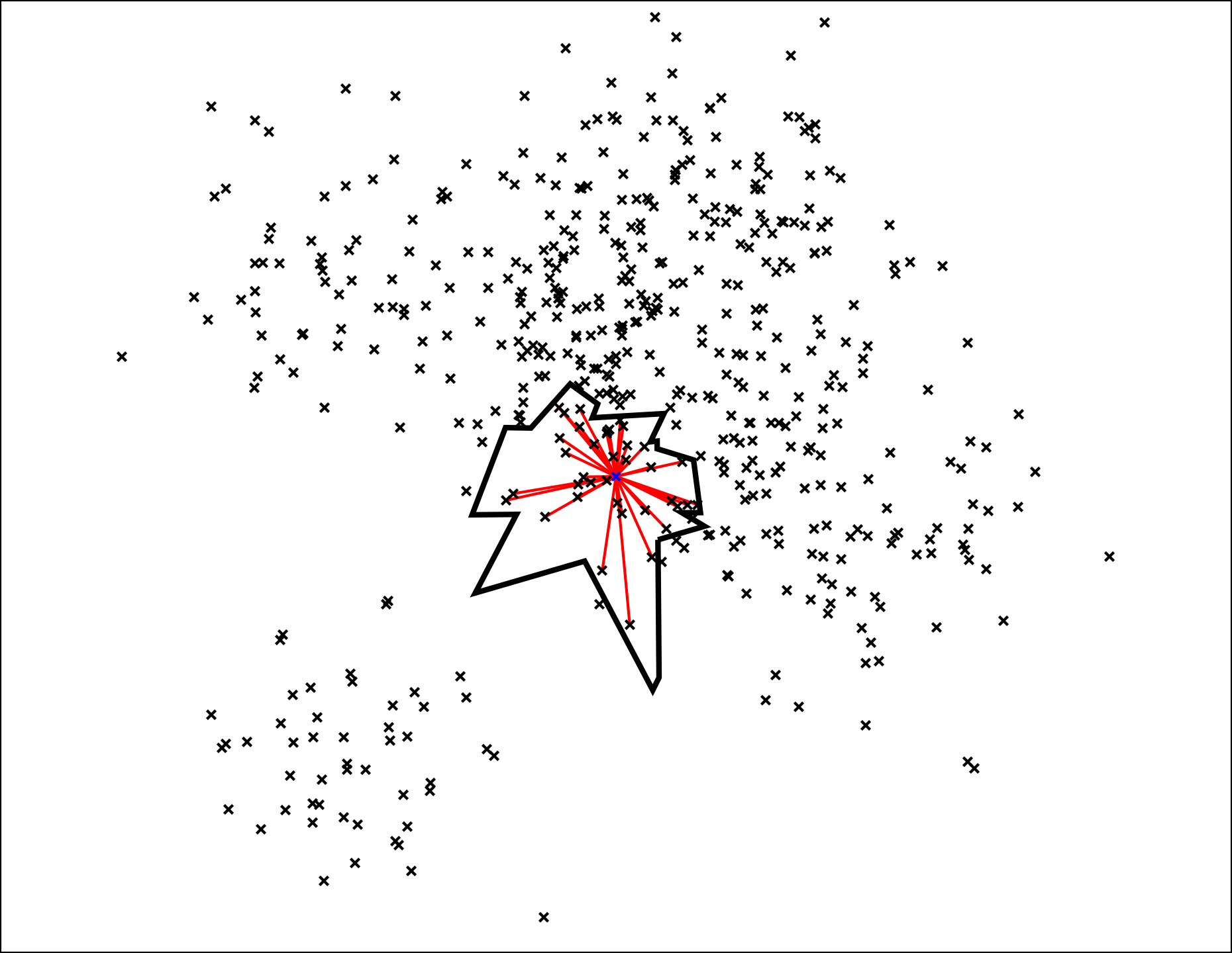
Trick 1 – use a priority queue
The trick we’re going to use is to go down on both sides of a split if we are “close enough” (which I will quantify in a second). So instead of just going down one path of the binary tree, we will go down a few more:
With the corresponding binary tree:
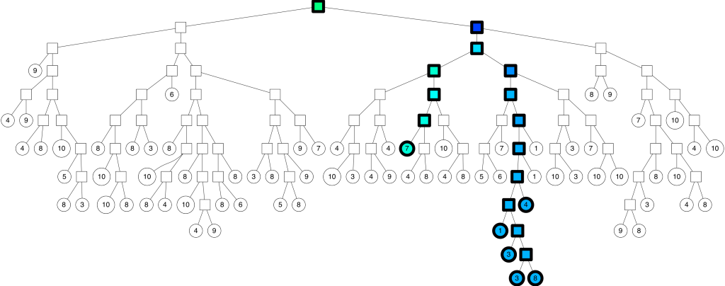
We can configure the threshold of how far we are willing to go into the “wrong” side of the split. If the threshold is 0, then we will always go on the “correct” side of the split. However if we set the threshold to 0.5 you get the search path above.
The trick here is we can actually use a priority queue to explore nodes sorted by the max distance into the “wrong” side. The nice part is we can search increasingly larger and larger thresholds starting from 0.
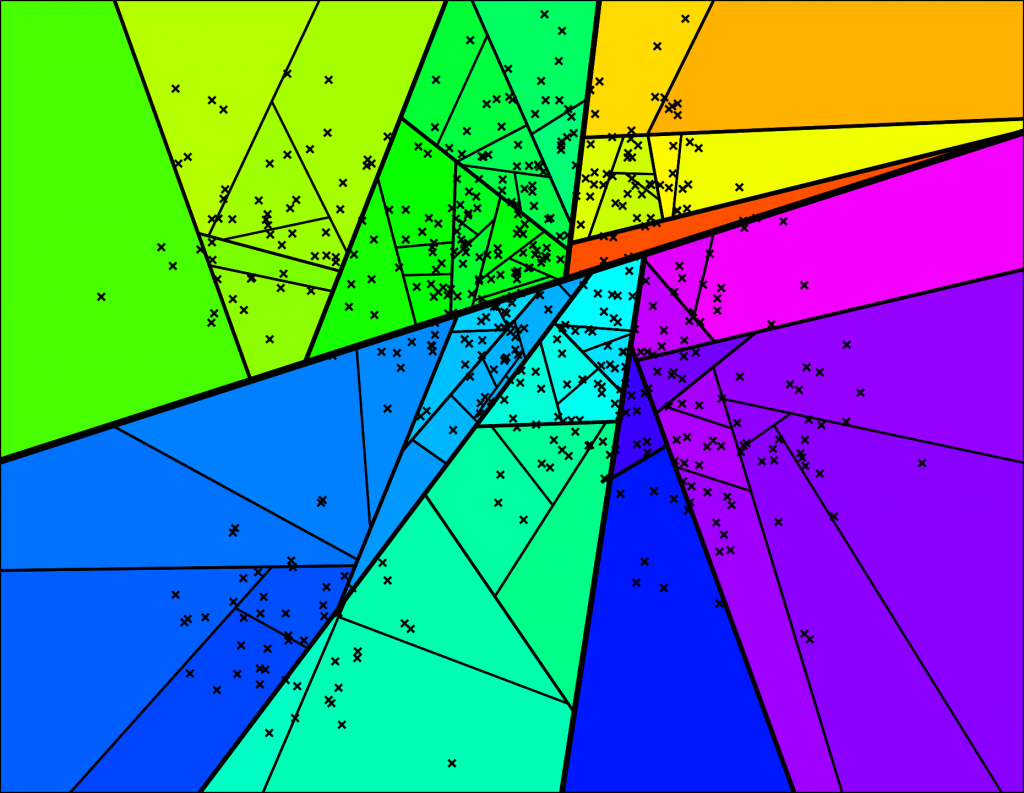
Trick 2 – build a forest of trees
The second trick we are going to use is is to construct many trees aka a forest. Each tree is constructed by using a random set of splits. We are going to search down all those trees at the same time:
We can search all trees at the same time using one single priority queue. This has an additional benefit that the search will focus on the trees that are “best” for each query – the splits that are the furthest away from the query point.
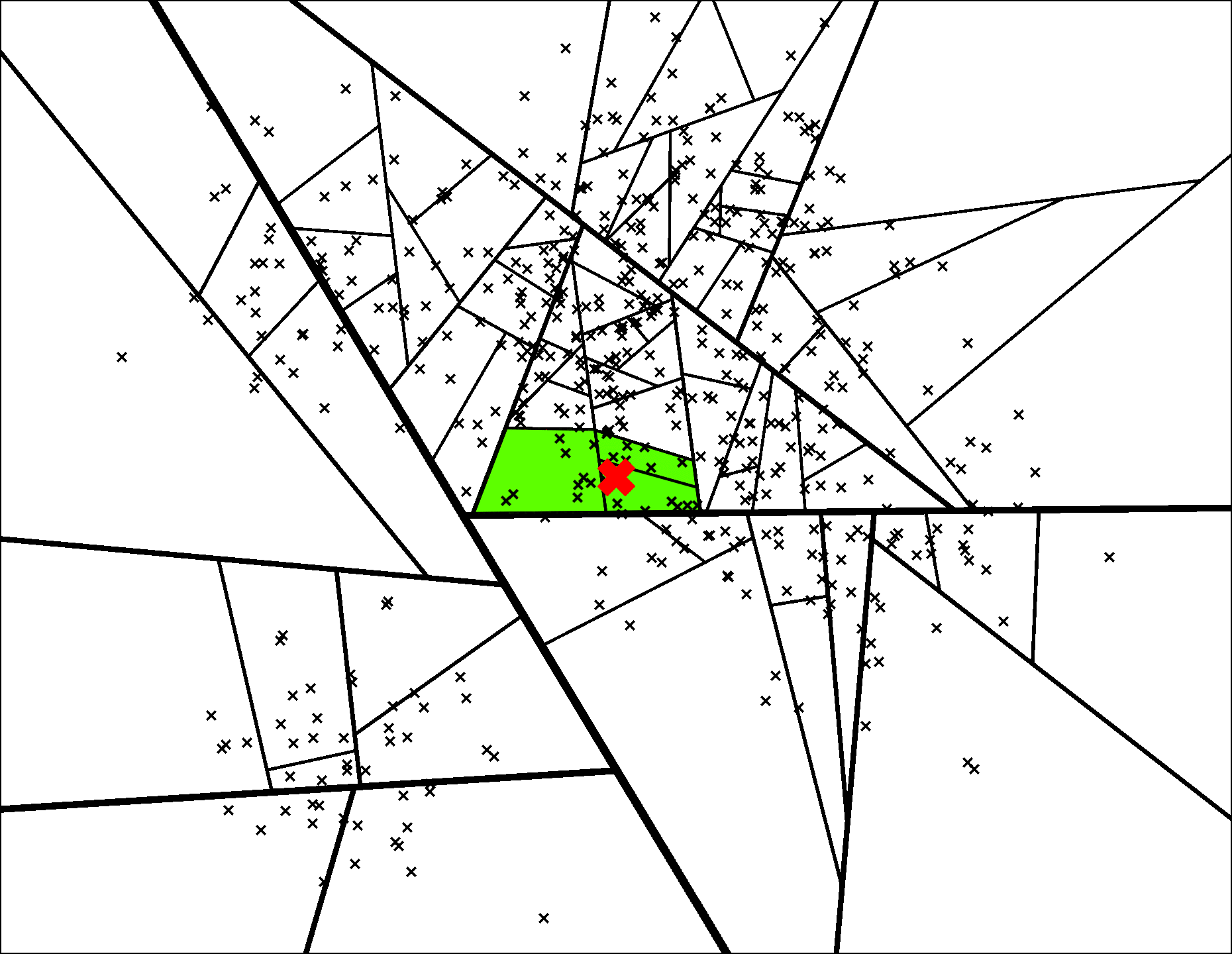
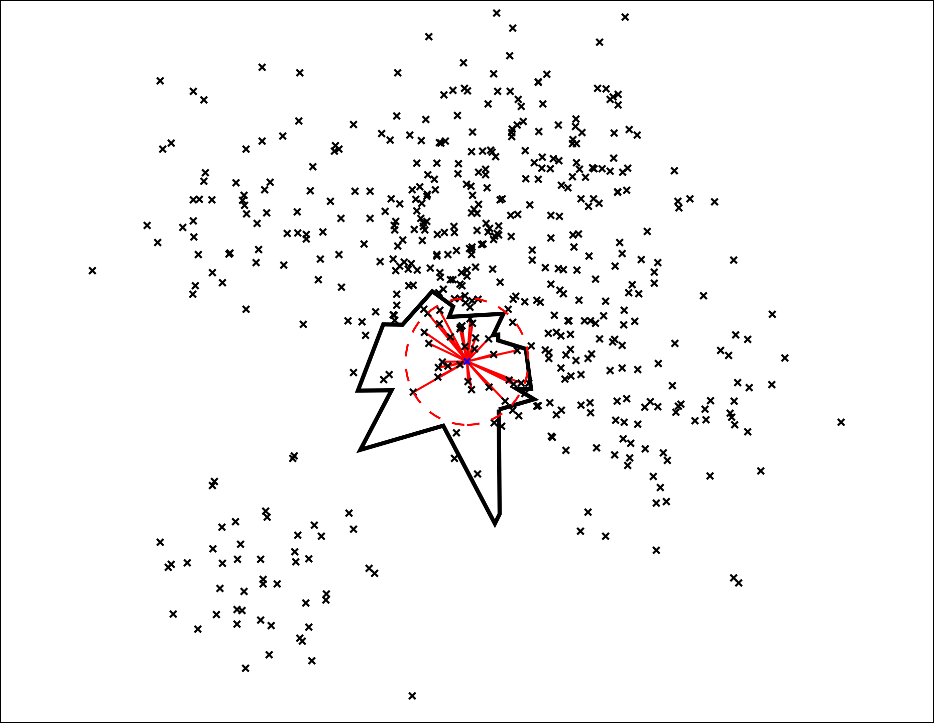
Every tree contains all points so when we search many trees we will find some points in multiple trees. If we look at the union of the leaf nodes we get a pretty good neighborhood:
At this point we have nailed it down to a small set of points. Notice so far we have not even computed distances to a single point. Next step is to compute all distances and rank the points:
We then sort all nodes by distance and return the top K nearest neighbors. Nice! And that is how the search algorithm works in Annoy.
Except one thing. In this case it turns out we actually did miss a couple of points outside:
But the A in Annoy stands for approximate and missing a few points is acceptable. Annoy actually has a knob you can tweak (search_k) that lets you trade off performance (time) for accuracy (quality).
The whole idea behind approximate algorithms is that sacrificing a little bit of accuracy can give you enormous performance gains (orders of magnitude). For instance we could return a decent solution where we really only computed the distance for 1% of the points – this is a 100x improvement over exhaustive search.
More trees always help. By adding more trees, you give Annoy more chances to find favorable splits. You generally want to bump it up as high as you can go without running out of memory.
Summary: Annoy’s algorithm
Preprocessing time:
- Build up a bunch of binary trees. For each tree, split all points recursively by random hyperplanes.
Query time:
- Insert the root of each tree into the priority queue
- Until we have _search_k _candidates, search all the trees using the priority queue
- Remove duplicate candidates
- Compute distances to candidates
- Sort candidates by distance
- Return the top ones
Feel free to check out _make_tree and _get_all_nns in annoylib.h
That’s it for this post! More is coming from the presentation shorly. Btw, the take a look at the slides, and the check out the code to generate all graphs in this post.
Tagged with: approximate nearest neighbors, math