Recurrent Neural Networks for Collaborative Filtering
I’ve been spending quite some time lately playing around with RNN’s for collaborative filtering. RNN’s are models that predict a sequence of something. The beauty is that this something can be anything really – as long as you can design an output gate with a proper loss function, you can model essentially anything.
In the case of collaborative filtering, we will predict the next item given the previous items. More specifically, we will predict the next artist, album, or track, given the history of streams. Without loss of generalization, let’s assume we want to predict tracks only.
Note that we’re not trying to predict ratings or any explicit information – just what track the user chose to play.
The data
We use playlist data or session data, because it has an inherent sequence to it. Removing consecutive duplicates improves performance a lot, since otherwise the network just learns to predict the same item as it just predicted.
In our case we use a few billion playlist/sessions and in total about ten to a hundred billion “words”.
The model
Recurrent neural networks have a simple model that tries to predict the next item given all previous ones. After predicting the item, the network gets to “know” what item it was, and incorporates this.
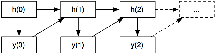
More formally, let’s assume we have time steps $$ 0 \ldots t-1 $$ . The model has a “hidden” internal state $$ h_0 \ldots h_{t-1} $$ . These are generally vectors of some dimension $$ k $$ . Every time step, we have two things going on
- Predict the output given the hidden state. We need to model a $$ P(y_i \mid h_i) $$ for this.
- Observe the output $$ y_t $$ and feed it back into the next hidden state $$ h_{i+1} $$ . In the most general form, $$ h_{i+1} = f(a(h_i) + b(y_i)) $$ . In practice, $$ f $$ is generally some nonlinear function like sigmoid or tanh, whereas $$ a $$ , and $$ b $$ are usually a simple linear transform. It depends a bit on the structure of the output.
Now, all we need to do is write down the total likelihood and optimize for it!
Wait a minute?
Sorry about the extremely superficial introduction without much detail. Here’s a more specific example:
Let’s say we want to predict a sequence of daily stock returns. In that case, $$ y_i $$ is a vector of stock returns – maybe containing three values with the daily return for Apple, Google, and Microsoft. To get from the hidden state $$ h_i $$ to $$ y_i $$ let’s just use a simple matrix multiplication: $$ y_i = W h_i $$
We can assume $$ P(y_i \mid h_i) $$ is a normal distribution because then the log-likelihood of the loss is just the (negative) L2 loss: $$ -(y_t - h_t)^2 $$
We can specify that $$ h_{i+1} = \tanh(Uy_i + Vh_i) $$ and that $$ h_0 = 0 $$ (remember it’s still a vector). If we want to be more fancy we could add bias terms and stuff but let’s ignore that for the purpose of this example. Our model is now completely specified and we have $$ 3k^2 $$ unknown parameters: $$ U $$ , $$ V $$ , and $$ W $$ .
What are we optimizing?
We want to find $$ U $$ , $$ V $$ , and $$ W $$ that maximizes the log-likelihood over all examples:
$$ \log L = \sum \limits_{\mbox{all examples}} \left( \sum \limits_{i=0}^{t-1} -(y_i - h_i)^2 \right) $$
Backprop
The way to maximize the log-likelihood is through back-propagation. This is a well-known method and there’s so much resources on line that I’ll be a bit superficial about the details.
Anyway, we need to do two passes through each sequence. First propagation. For $$ i=0 \ldots t-1 $$ : Calculate all hidden states $$ h_i $$ . Nothing magic going on here, we’re just applying our rule.
Now it’s time for backprop. This is essentially just the chain rule taken to the extreme. Remember that the total log-likelihood is the sum of all the individual log-probabilities of observing each output:
$$ L = \sum \limits_{i=0}^{t-1} \log P(y_i \mid h_i) $$
We define the derivatives $$ \delta_i $$ as the partial derivatives of the log-likelihood with respect to the hidden state:
$$ \delta_i = \frac{\partial \log L}{\partial h_i} $$
Since each hidden state only influences later hidden states, the $$ \delta $$’s are just a function of all future $$ \delta_j, j = i \ldots t-1 $$ .
$$ \delta_i = \sum \limits_{j=i}^{t-1}\frac{\partial \log P(y_j \mid h_j)}{\partial h_i} $$
We can now rewrite $$ \delta_i $$ as a function of $$ \delta_{i+1} $$ and use some chain rule magic:
$$ \frac{\partial \log L}{\partial h_i} = \delta_i = \frac{\partial}{\partial h_i} \log P(y_i \mid h_i) + \frac{\partial h_{i+1}}{\partial h_{i}} \delta_{i+1} $$
We can evaluate this backwards from $$ t-1 \ldots 0 $$ . Both $$ P(y_i \mid h_i) $$ and $$ \frac{\partial h_{i+1}}{\partial h_{i}} $$ are specified by our model, so we just need to plug in the expressions.
For the stock price example, we have the unknown parameters $$ U, V, W $$ where we can derive the gradients like this:
- $$ \frac{\partial \log L}{\partial U} = \frac{\partial L}{\partial h_{i+1}}\frac{\partial h_{i+1}}{\partial U} = \delta_{i+1} \frac{\partial}{\partial U} \tanh(Uy_i + Vh_i) = \delta_{i+1} \tanh’(Uy_i + Vh_i) y_i^T $$
This looks intimidating but it’s really just a lot of chain rule applications and fairly straightforward math. You get similar gradients for $$ V, W $$ . Now that we have the gradients, we can optimize using stochastic gradient descent over lots of example.
How does this relate to Hidden Markov Models?
The nice thing about RNN’s is that the relation between $$ h_{t+1} $$ and $$ h_t $$ is exact rather than being some probabilistic relationship. This means that the $$ h $$ ‘s are not parameters in themselves, so we don’t have to solve for them at all. This is usually the slow part of HMM’s since figuring out the hidden values takes some slow iterative process like the Baum-Welch algorithm. For RNN’s, we only need two passes through each sequence rather than iterating lots of times until the hidden states converge.
The other thing is that RNN’s need some kind of nonlinearity or else they magnitude of the hidden states will explode. This nonlinearity is usually taken to be sigmoid or tanh. I guess in theory HMM’s could also use nonlinearities, but I’ve never heard of this.
Predicting other things
Let’s focus on the collaborative filtering example. Given a sequence of watched movies, or tracks that the user has listened to, predict what the next one is going to be. Now $$ y_i $$ is not a scalar, but one out of many items. We need some kind of distribution $$ P(y_i \mid h_i) $$ . The one I’ve seen being used is the Softmax distribution over all possible outputs. This means we have to learn a vector $$ a_j $$ for each item. The probability $$ P(y_i \mid h_i) $$ is now proportional to $$ \exp(h_t^Ta_j) $$ :
$$ P(y_i \mid h_i) = \frac{\exp(h_t^Ta_j)}{\sum_k \exp(h_t^Ta_k)} $$
Notice that the summation part in the denominator is over all items – something that is pretty slow to compute. I’ll get back to that.
We also need something linking back the output to the next hidden state. In fact, we will learn another set of vectors $$ b_j $$ – one for each item. With slight abuse of notation, here is how it looks like:
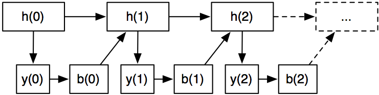
Since we are learning a bunch of vectors, we don’t need the matrices $$ U $$ and $$ V $$ . Our model now becomes:
$$ h_{i+1} = \tanh(W h_i + b_i) $$
with some slight abuse of notation since the $$ b $$ ‘s are shared for each item $$ y_i $$ . Again, we want to maximize the total log-likelihood
$$ \sum \sum_{i=0}^t \log P(y_i \mid h_i) $$
We now end up with a ton of parameters because we have the unknowns $$ a_j $$ ‘s and $$ b_j $$ ‘s for each item.
Let’s just pause here and reflect a bit: so far this is essentially a model that works for any sequence of items. There’s been some research on how to use this for natural language processing. In particular, check out Tomas Mikolov’s work on RNN’s (this is the same guy that invented word2vec, so it’s pretty cool.
The gnarly details
If you have 10 different items, you can evaluate $$ P(y_i \mid h_i) $$ easily, but not if you have five million items. But do not despair! There’s a lot of ways you can attack this:
- Take the right output and sample some random items from the entire “vocabulary”. Train the model to classify which one is the right output. This is sort of like a police lineup: one is the right suspect, the remaining people just some random sample.
- Hierarchical softmax: Put all items in a binary tree, and break it up into roughly $$ \log m $$ binary classification problems (where m is the size of the vocabulary).
Instead of messing around with Hamming trees and things recommended in literature, I ended up implementing a much more simple version of hierarchical softmax. Internally, all item are described as integers, so I build the tree implicitly. The root node is a binary classifier for the last bit of the item. The next level classifies the second last bit, and so on.
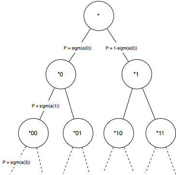
The idea is that you can calculate $$ P(y_i \mid h_i) $$ as the product of all the probabilities for each individual node on the path from the root to the leaf.
Instead of learning an $$ a_j $$ for every item, we just have to learn one for every node in the tree, in total $$ 2^{\lceil{log_2 m}\rceil -1} $$ vectors. It doesn’t really matter that much how we build the tree – we don’t need to enforce that similar items are close to each other in the tree (however that would probably improve performance a bit).
But in general, this problem pops up in a lot of places and here’s some other crazy ideas I’ve thought about:
- If generating random “negative” samples, one way to better mine random examples would be to sample some items from the $$ y_i $$ ‘s themselves. Since those values are probably pretty similar, that would force the model to discriminate between more “hard” cases.
- Assume the $$ a_j $$ ‘s have some kind of distribution like a Normal distribution, and calculate an expectation. This is just a bunch of integrals. We’ve had some success using this method in other cases.
- Don’t use softmax but instead use L2 loss on $$ m $$ binary classification problems. All entries would be $$ 0 $$ except the right one which is $$ 1 $$ . You can put more weight on the right one to address the class imbalance. The cool thing is that with L2 loss, everything becomes linear, and you can compute the sum over all items in constant time. This is essentially how Yehuda Koren’s 2008 paper on implicit collaborative filtering works
Implementing it
I ended up building everything in C++ because it’s fast and I’m pretty comfortable with it. It reads about 10k words per second on a single thread. A multi-threaded version I’ve built can handle 10x that amount and we can parse 10B “words” in about a day.
Hyperparameters
A beautiful thing with this model is that there’s basically no hyperparameters. The larger number of factors is better – we typically use 40-200. With dropout (see below) overfitting is not a concern. It takes a little trial and error to get the step sizes right though.
Initialization
As with most latent factor models, you need to initialize your parameter to random noise. Typically small Gaussian noise like $$ \mathcal{N}(0, 0.1^2) $$ works well.
Nonlinearity
I tried both sigmoid and tanh. Tanh makes more sense to me, because it’s symmetric around 0, so you don’t have to think too much about the bias term. Looking at some offline benchmarks, it seemed like tanh was slightly better than sigmoid.
Dropout
I also added dropout to the hidden values since it seemed to help improve the predictions of the model. After the each $$ h_i $$ is calculated, I set half of them to zero. This also seems to help with exploding gradients. What happens is that the $$ W $$ matrix will essentially learn how to recombine the features
Gradient clipping
Actually gradient clipping wasn’t needed for sigmoid, but for tanh I had to add it. Basically during the backprop I cap the magnitude of the gradient to 1. This also helps equalizing the impact of different examples since otherwise for longer sequences you get bigger gradients.
Adagrad
I use Adagrad on the item vectors but simple learning rate on the shared parameters $$ W $$ and the bias terms. Adagrad is fairly simple: in addition to each vector $$ a_j $$ and $$ b_j $$ you just store a single scalar with the sum of the squared magnitudes of the gradients. You then use that to normalize the gradient.
For a vector $$ x $$ with gradient $$ d $$ , Adagrad can be written as:
$$ x^{(n+1)} = x^{(n)} + \eta \frac{d^{(n)}}{\sqrt{\sum \limits_{i=1 \ldots n} \left( d^{(i)} \right)^2}} $$
$$ \eta $$ is a hyperparameter that should be set to about half the final magnitude these vectors will have. I usually have had success just setting $$ \eta = 1 $$ .
Results
Offline results show that the RNN is one of the best performing algorithms for collaborative filtering and A/B tests confirm this.
More resources
I can recommend A tutorial on training recurrent neural networks as another starting point to read more about recurrent neural networks.
(Edit: fixed some minor errors in the math and a wrong reference to Baum-Welch)
Tagged with: math