Nearest neighbor methods and vector models – part 1
This is a blog post rewritten from a presentation at NYC Machine Learning last week. It covers a library called Annoy that I have built that helps you do (approximate) nearest neighbor queries in high dimensional spaces. I will be splitting it into several parts. This first talks about vector models, how to measure similarity, and why nearest neighbor queries are useful.
Nearest neighbors refers to something that is conceptually very simple. For a set of points in some space (possibly many dimensions), we want to find the closest k neighbors quickly.
This turns out to be quite useful for a bunch of different applications. Before we get started on exactly how nearest neighbor methods work, let’s talk a bit about vector models.
Vector models and why nearest neighbors are useful
Vector models are increasingly popular in various applications. They have been used in natural language processing for a long time using things like LDA and PLSA (and even earlier using TF-IDF in raw space). Recently there has been a new generation of models: word2vec, RNN’s, etc.
In collaborative filtering vector models have been among the most popular methods since going back to the Netflix Prize – the winning entry featured a huge ensemble where vector models made up a huge part.
The basic idea is to represent objects in a space where proximity means two items are similar. If we’re using something like word2vec it could look something like this:
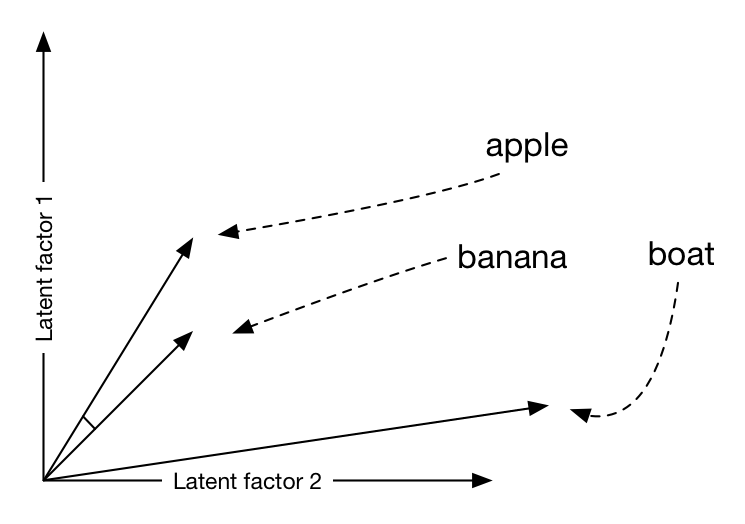
In this case similarity between words is determined by the angle between them. apple and banana are close to each other, whereas boat is further.
(As a side note: much has been written about word2vec’s ability to do word analogies in vector space. This is a powerful demonstration of the structure of these vector spaces, but the idea of using vector spaces is old and similarity is arguably much more useful).
In the most basic form, data is already represented as vectors. For an example of this, let’s look at one of the most canonical data sets in machine learning – the MNIST handwritten digits dataset.
Building an image search engine for handwritten digits
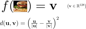
The MNIST dataset features 60,000 images of size 28×28. They each feature a handwritten digits in grayscale. One of the most basic ways we can play around with this data set is to smash each 28×28 array into a 784-dimensional vector. There is absolutely no machine learning involved in doing this, but we will get back and introduce cool stuff like neural networks and word2vec later.
Let’s define a distance function in this space. Let’s say the distance between two digits is the squared sum of the pixel differences. This is basically the squared Euclidean distance (i.e. the good old Pythagorean theorem):
This is nice because we can compute the distance of arbitrary digits in the dataset:
This now lets us search for neighbors in this 784-dimensional space. Check out some samples below – the leftmost digit is the seed digit and to the right of it are the ten most similar images using the pixel distance.
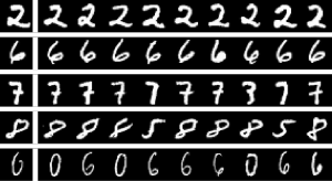
You can see that it sort of works. The digits are visually quite similar, although it’s obvious to a human that some of the nearest neighbors are the wrong digit.
This was pretty nice and easy, but this also an approach that doesn’t scale very well. What about larger images? What about color images? And how to we determine similars not just in terms of visual similarity but actually what a human would think of as similar. This simple definition of “distance” leaves a lot of room for improvement.
Dimensionality reduction
A powerful method that works across a wide range of domains is to take high dimensional complex items and project the items down to a compact vector representation.:
- Do a dimensionality reduction from a large dimensional space to a small dimensional space (10-1000 dimensions)
- Use similarity in this space instead
Dimensionality reduction is an extremely powerful technique because it lets us take almost any object and translate it to a small convenient vector representation in a space. This space is generally referred to as latent because we don’t necessarily have any prior notion of what the axes are. What we care about is that objects that are similar end up being close to each other. What do we mean with similarity? In a lot of cases we can actually discover that from our data.
So let’s talk about one approach for dimensionality reduction on images: deep convolutional neural networks. I had a side project about a year ago to classify food. It’s a pretty silly application but the eventual goal was to see if you could predict calorie content from pictures, and a side goal was to learn how to use convolutional neural networks. I never ended up using this for anything and wasted way to much money renting GPU instances on AWS, but it was fun.
To train the model, I downloaded 6M pics from Yelp and Foursquare and trained a network quite similar to the one described in this paper using Theano.
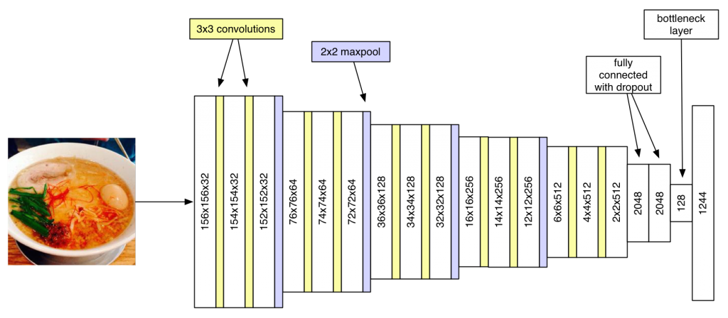 ](/assets/2015/09/foodnet.png)
The final layer in this model is a 1244-way multi-classification output using softmax so we’re training this in a supervised way. These are words that occurred in the description text, eg. “spicy ramen” for the one above. However the nice thing is we have a “bottleneck” layer just before the final layer – a 128-dimensional vector that gives us exactly what we want.
Using the neural network as an embedding function and using cosine similarity as a metric (this is basically Euclidean distance, but normalize the vectors first) we get some quite cool nearest neighbors:
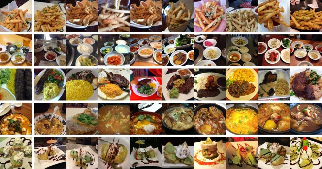
These similars look pretty reasonable! The top left picture is similar to a bunch of other fries. The second row shows a bunch of different white bowls with Asian food – more impressively they are all in different scales and angles, and pixel by pixel similarity is quite low. The last row shows a bunch of desserts with similar patterns of chocolate sprinkled over it. We’re dealing with a space that can express object features quite well.
So how do we do find similar items? I’m not going to describe dimensionality reduction in great detail – there are a million different ways that you can read about. What I have spent more time thinking about is how to search for neighbors in vector spaces. In fact, finding the neighbors above takes only a few milliseconds per picture, because Annoy is very fast. This is why dimensionality reduction is so extremely useful. At the same time that it’s discovering high level structure in data, it also computes a compact representation of items. This representation makes it easy to compute similarity and search for nearest neighbors.
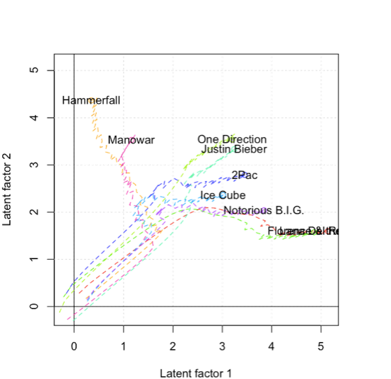
Vector methods in collaborative filtering
Reducing dimensionality isn’t just useful in computer vision, of course. As mentioned, it’s incredibly useful in natural language processing. At Spotify, we use vector models extensively for collaborative filtering. The idea is to project artists, users, tracks, and other objects into a low dimensional space where similarity can be computed easily and recommendations can be made. This is in fact what powers almost all of the Spotify recommendations – in particular Discover Weekly that was launched recently.

I have already put together several presentations about this so if you’re interested, you should check out some of them:
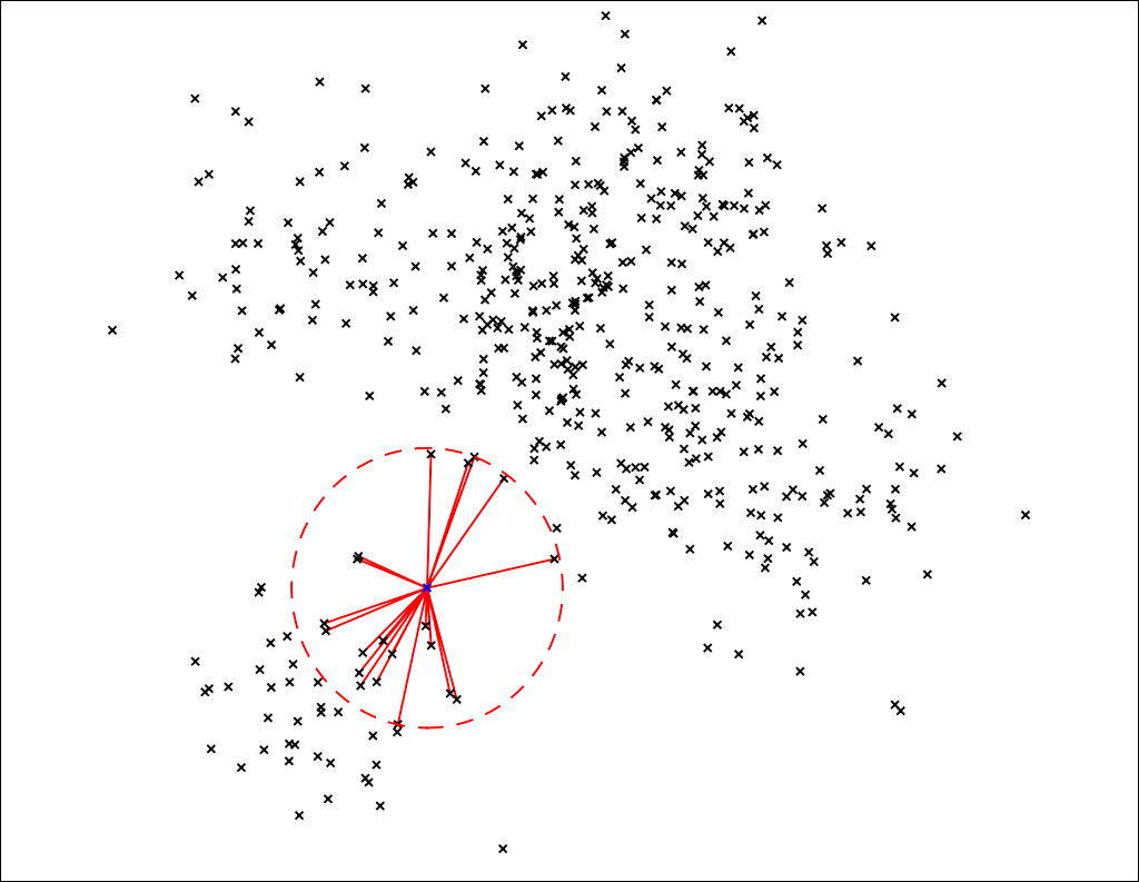
Exhaustive search as a baseline
So how do we find similar items? Before we go into detail about how Annoy works, it’s worth looking at the baseline of doing a brute force exhaustive search. This means iterating over all possible items and computing the distance for each one of them to our query point.
word2vec actually comes with a tool to do exhaustive search. Let’s see how it compares! Using the GoogleNews-vectors-negative300.bin dataset and querying for “chinese river”, it takes about 2 minutes 34 seconds to output this:
- Qiantang_River
- Yangtse
- Yangtze_River
- lake
- rivers
- creek
- Mekong_river
- Xiangjiang_River
- Beas_river
- Minjiang_River
I wrote a similar tool that uses Annoy (available on Github here). The first time you run it, it will precompute a bunch of stuff and can take a lot of time to run. However the second time it runs it will load (mmap) an Annoy index directly from disk into memory. Relying on the magic page cache, this will be very fast. Let’s take it for a spin and search for “chinese river”:
- Yangtse
- Yangtze_River
- rivers
- creek
- Mekong_river
- Huangpu_River
- Ganges
- Thu_Bon
- Yangtze
- Yangtze_river
Amazingly, this ran in 470 milliseconds, probably some of it overhead for loading the Python interpreter etc. This is roughly 300x faster than the exhaustive search provided by word2vec.
Now – some of you probably noticed that the results are marginally different. That’s because the A in Annoy stands for approximate. We are deliberately trading off some accuracy in return for a huge speed improvement. It turns out you can actually control this knob explicitly. Telling Annoy we want to search through 100k nodes (will get back to that later) we get this result in about 2 seconds:
- Qiantang_River
- Yangtse
- Yangtze_River
- lake
- rivers
- creek
- Mekong_river
- Xiangjiang_River
- Beas_river
- Minjiang_River
This is exactly the same as the exhaustive search it turns out – and still about 50x faster.
Other uses of nearest neighbors
Finally just as a fun example of another use, nearest neighbors is useful when you’re dealing with physical spaces too. In an earlier blog post, I was showing this world map of how long it takes to ping IP addresses from my apartment in NYC:
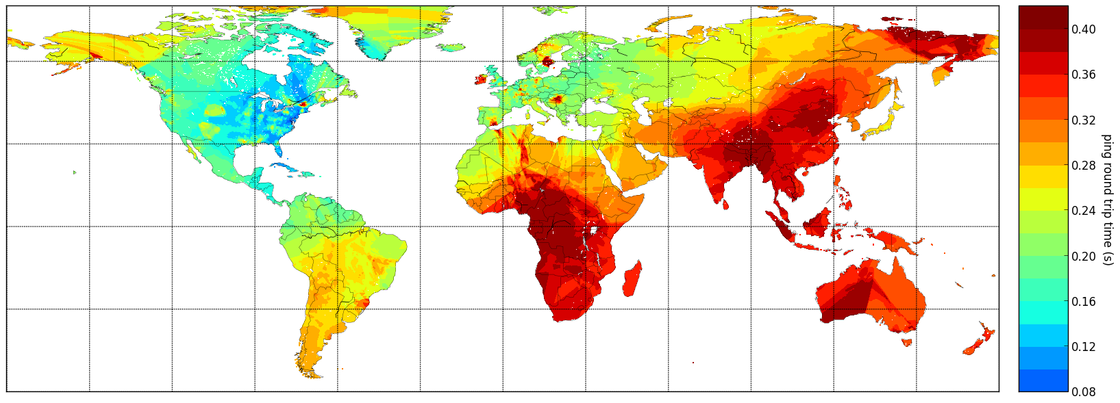
This is a simple application of k-NN (k-nearest neighbors) regression that I’ve written earlier about on this blog. There is no dimensionality reduction involved here – we just deal with 3D coordinates (lat/long projected to the unit sphere).
In the next series, I will go in depth about how Annoy works. Stay tuned!
Tagged with: approximate nearest neighbors, math