Nearest neighbors and vector models – epilogue – curse of dimensionality

This is another post based on my talk at NYC Machine Learning. The previous two parts covered most of the interesting parts, but there are still some topics left to be discussed. To go back and read the meaty stuff, check out

• Part 1: What are vector models useful for?
• Part 2: How to search in high dimensional spaces – algorithms and data structures

You should also check out the slides and the video if you're interested. Anyway, let's talk about the curse of dimensionality today.

This pic was obviously worth spending 20 minutes on

Curse of dimensionality refers to a set of things that happen when you are dealing with items in high dimensional spaces, in particular what happens with distances and neighborhoods, in such a way that finding the nearest neighbors gets tricky.

Consider a map of the world. Most countries have a handful of neighboring countries. It is also pretty close from New York to Philadelphia but it's far from New York to Beijing – distances are very different.

What happens when we go to higher dimensions is that everything starts being close to everything. All cities end up having almost the same distance to each other and all countries have borders to all other countries (Trump would have a lot of walls to build). This is highly nonintuitive (as is anything with more than 3 dimensions) but let's try to quantify this.

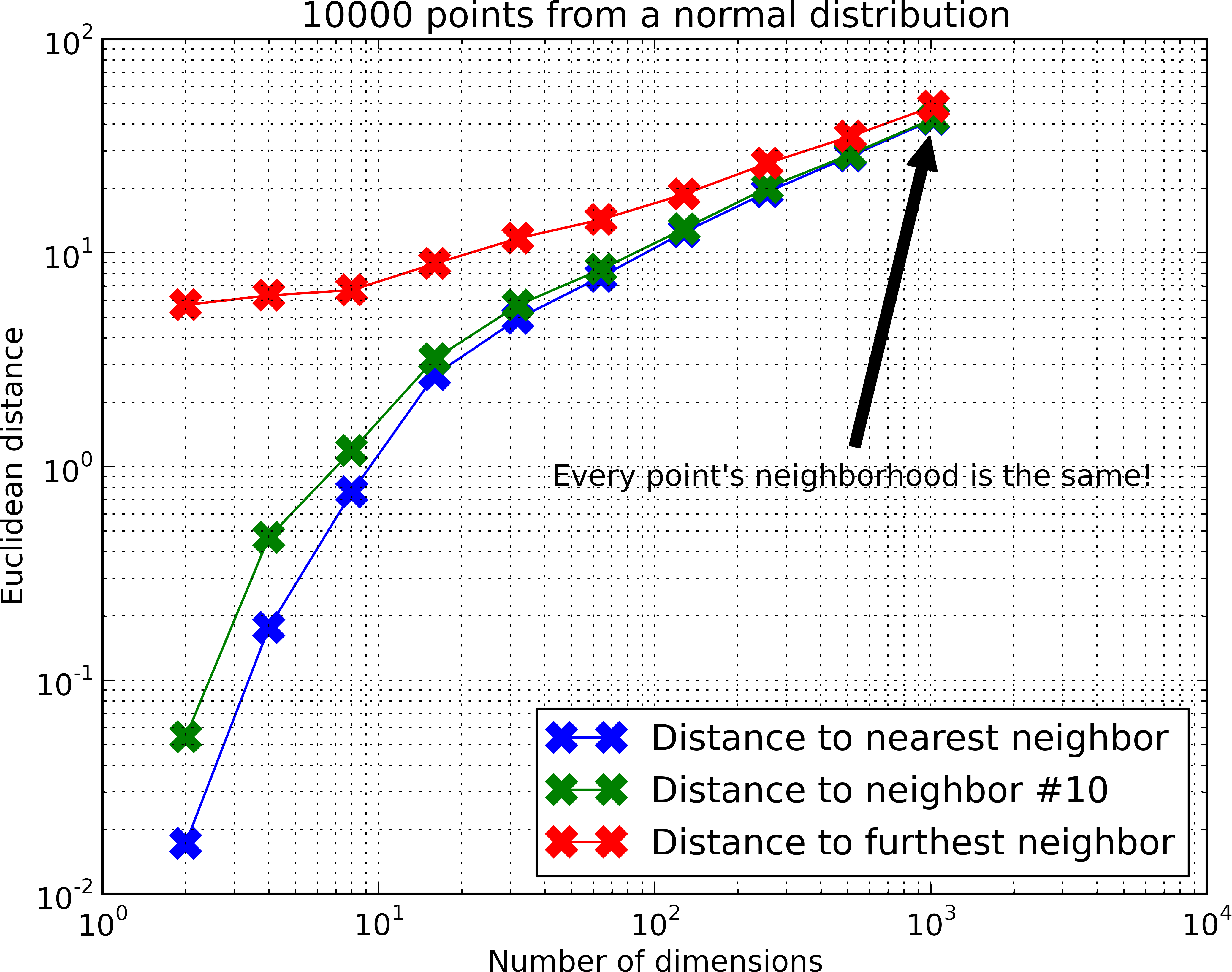
Let's look at how distances behaves as we go to higher dimensions. Let's sample a 10,000 points from a normal distribution, then pick a random point in the distribution, and compute the distance to the furthest and closest point:

(For code, check out knn_avg_dist.py on Github)

As the number of dimensions increase, the distances to the closest and the furthest point are almost similar. Wikipedia's article is actually quite enlightening and features this statement that as we go to higher dimensions, we have the relationship:

$$ \huge \lim_{d \to \infty} E\left(\frac{\text{dist}_{\max} (d) - \text{dist}_{\min} (d)}{\text{dist}_{\min} (d)}\right) \to 0 $$

For example if we are in a high dimensional version of New York, then the nearest city is 1.000 miles away and the furthest city is 1.001 miles away. The ratio above is then 0.001. Let's get back to this ratio shortly.

This weird behavior makes nearest neighbors in high dimensional spaces tricky. It's still an open problem whether exact k-NN is solvable in polynomial time.

Saving the day

The above relation applies to distribution where there is little structure – in particular the example I generated was just data points from the normal distribution. In the real world data sets we usually have a lot of structure in our data. Consider all the cities and towns of the world. This is a set of points in in 3D space, but all cities lie on a 2D sphere and so the point set will actually behave more 2D-like.

The same thing happens to word embeddings or any other set of vectors. Even if we're dealing with 1000's of dimensions, there underlying structure is really much more lower dimensional. This is exactly why dimensionality reduction works so well!

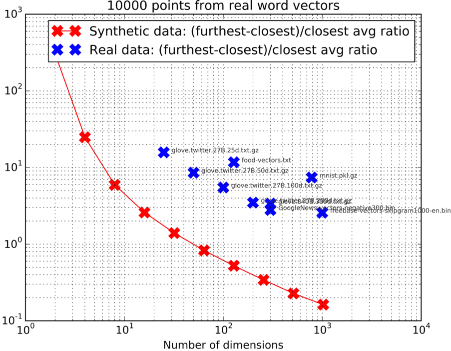
Let's actually compute the quantity mentioned above and map out some real datasets:

(Again for the code, check out knn_avg_dist.py on Github)

The graph above shows something pretty interesting: some of these “real” high dimensional data sets have a ratio that is similar to much fewer dimensions for the normal distribution.

Look at the Freebase vectors (which you can download here) for instance – they are 1000D, but they are similar to a normal distribution in 16D in terms of the ratio. This behavior holds true for a whole set of different vectors. The 784-dimensional MNIST digits data set behaves as the 8D normal distribution. The 128-dimensional embedding of food pictures same thing.

I think this is why approximate nearest neighbor methods work so well up to thousands of dimensions. The key thing is the algorithms need to learn the distribution from the data. I am generally bearish on LSH for this reason.

Enough about approximate nearest neighbors for a while! Hope you liked this series of posts!