Why software projects take longer than you think: a statistical model
Anyone who built software for a while knows that estimating how long something is going to take is hard. It’s hard to come up with an unbiased estimate of how long something will take, when fundamentally the work in itself is about solving something. One pet theory I’ve had for a really long time, is that some of this is really just a statistical artifact.
I suspect devs are actually decent at estimating the *median* time to complete a task. Planning is hard because they suck at the *average*.
— Erik Bernhardsson (@bernhardsson) May 11, 2017
Let’s say you estimate a project to take 1 week. Let’s say there are three equally likely outcomes: either it takes 1/2 week, or 1 week, or 2 weeks. The median outcome is actually the same as the estimate: 1 week, but the mean (aka average, aka expected value) is 7/6 = 1.17 weeks. The estimate is actually calibrated (unbiased) for the median (which is 1), but not for the the mean.
A reasonable model for the “blowup factor” (actual time divided by estimated time) would be something like a log-normal distribution. If the estimate is one week, then let’s model the real outcome as a random variable distributed according to the log-normal distribution around one week. This has the property that the median of the distribution is exactly one week, but the mean is much larger:
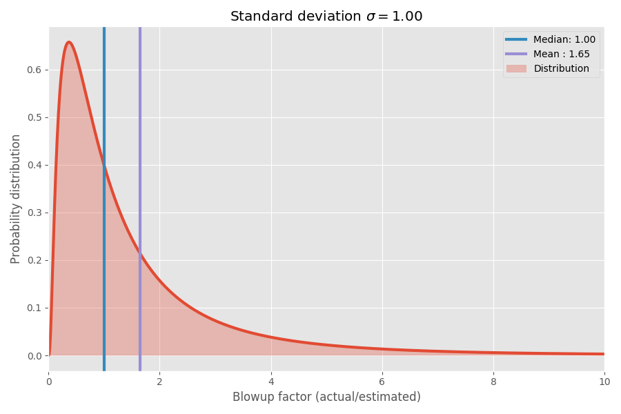
If we take the logarithm of the blowup factor, we end up with a plain old normal distribution centered around 0. This assumes the median blowup factor is 1x, and as you hopefully remember, log(1) = 0. However, different tasks may have different uncertainties around 0. We can model this by varying the σ parameter which corresponds to the standard deviation of the normal distribution:
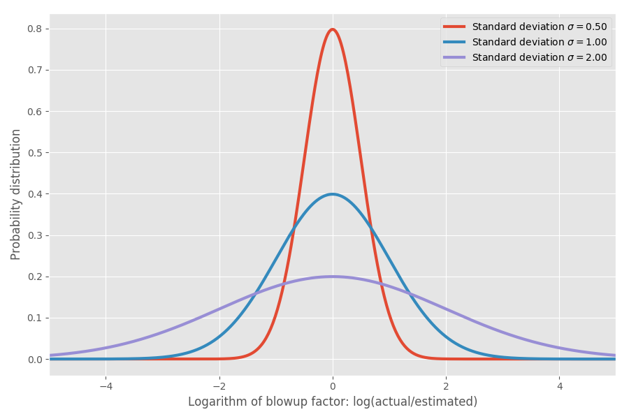
Just to put some numbers on this: when log(actual / estimated) = 1 then the blowup factor is exp(1) = e = 2.72. It’s equally likely that a project blows up by a factor of exp(2) = 7.4 as it is that it completes in exp(-2) = 0.14 i.e. completes in 14% of the estimated time. Intuitively the reason the mean is so large is that tasks that complete faster than estimated have no way to compensate for the tasks that take much longer than estimated. We’re bounded by 0, but unbounded in the other direction.
Is this just a model? You bet! But I’ll get to real data shortly and show that this in fact maps to reality reasonably well using some empirical data.
Software estimation
So far so good, but let’s really try to understand what this means in terms of software estimation. Let’s say we look at the roadmap and it consists of 20 different software projects and we’re trying to estimate: how long is it going to take to complete all of them.
Here’s where the the mean becomes crucial. Means add, but medians do not. So if we want to get an idea of how long it will take to complete the sum of n projects, we need to look at the mean. Let’s say we have three different projects in the pipeline with the exact same σ = 1:
| Median | Mean | 99% | |
|---|---|---|---|
| Task A | 1.00 | 1.65 | 10.24 |
| Task B | 1.00 | 1.65 | 10.24 |
| Task C | 1.00 | 1.65 | 10.24 |
| SUM | 3.98 | 4.95 | 18.85 |
Note that the means add up and 4.95 = 1.65*3, but the other columns don’t.
Now, let’s add up three projects with different sigmas:
| Median | Mean | 99% | |
|---|---|---|---|
| Task A (σ = 0.5) | 1.00 | 1.13 | 3.20 |
| Task B (σ = 1) | 1.00 | 1.65 | 10.24 |
| Task C (σ = 2) | 1.00 | 7.39 | 104.87 |
| SUM | 4.00 | 10.18 | 107.99 |
The means still add up, but are nowhere near the naïve 3 week estimate you might come up with. Note that the high-uncertainty project with σ=2 basically ends up dominating the mean time to completion. For the 99% percentile, it doesn’t just dominate it, it basically absorbs all the other ones. We can do a bigger example:
| Median | Mean | 99% | |
|---|---|---|---|
| Task A (σ = 0.5) | 1.00 | 1.13 | 3.20 |
| Task B (σ = 0.5) | 1.00 | 1.13 | 3.20 |
| Task C (σ = 0.5) | 1.00 | 1.13 | 3.20 |
| Task D (σ = 1) | 1.00 | 1.65 | 10.24 |
| Task E (σ = 1) | 1.00 | 1.65 | 10.24 |
| Task F (σ = 1) | 1.00 | 1.65 | 10.24 |
| Task G (σ = 2) | 1.00 | 7.39 | 104.87 |
| SUM | 9.74 | 15.71 | 112.65 |
Again, one single misbehaving task basically ends up dominating the calculation, at least for the 99% case. Even for mean though, the one freak project ends up taking over roughly half the time spend on these tasks, despite all of these tasks having a similar median time to completion. To make it simple, I assumed that all tasks have the same estimated size, but different uncertainties. The same math applies if we vary the size as well.
Funny thing is I’ve had this gut feeling for a while. Adding up estimates rarely work when you end up with more than a few tasks. Instead, figure out which tasks have the highest uncertainty – those tasks are basically going to dominate the mean time to completion.
I have two methods for estimating project size:
— Erik Bernhardsson (@bernhardsson) March 8, 2019
(a) break things down into subprojects, estimate them, add it up
(b) gut feeling estimate based on how nervous i feel about unexpected risks
So far (b) is vastly more accurate for any project more than a few weeks
A chart summarizes the mean and 99th percentile as a function of the uncertainty (σ):
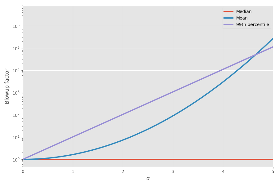
There is math to this now! I’ve started appreciating this during project planning: I truly think that adding up task estimates is a really misleading picture of how long something will take, because you have these crazy skewed tasks that will end up taking over.
Where’s the empirical data?
I filed this in my brain under “curious toy models” for a long time, occasionally thinking that it’s a neat illustration of a real world phenomenon I’ve observed. But surfing around on the interwebs one day, I encountered an interesting dataset of project estimation and actual times. Fantastic!
Let’s do a quick scatter plot of estimated vs actual time to completion:
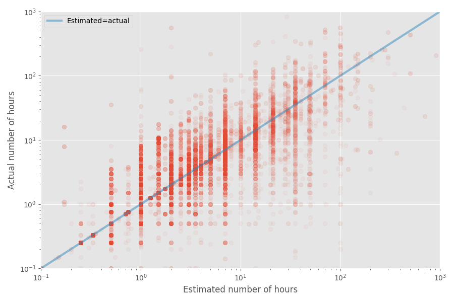
The median blowup factor turns out to be exactly 1x for this dataset, whereas the mean blowup factor is 1.81x. Again, this confirms the hunch that developers estimate the median well, but the mean ends up being much higher.
Let’s look at the distribution of the blowup factor. We’re going to look at the logarithm of it:
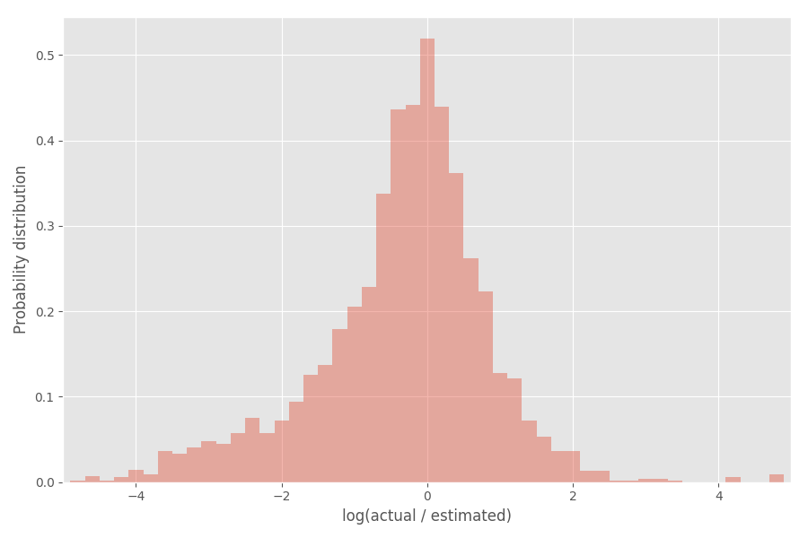
You can see that it’s pretty well centered around 0, where the blowup factor is exp(0) = 1.
Let’s go grab the statistics toolbox
I’m going to get a bit fancy with statistics now – feel free to skip if it’s not your cup of tea. What can we infer from this empirical distribution? You might expect that the logarithms of the blowup factor would distribute according to a normal distribution, but that’s not quite true. Note that the σs are themselves random and vary for each project.
One convenient way to model the σs is that they are sampled from an inverse Gamma distribution. If we assume (like previously) that the log of the blowup factors are distributed according to a normal distribution, then the “global” distribution of the logs of blowup factors ends up being Student’s t-distribution.
Let’s fit a Student’s t-distribution to the distribution above:
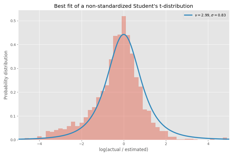
Decent fit, in my opinion! The parameters of the t-distribution also define the inverse Gamma distribution of the σ values:
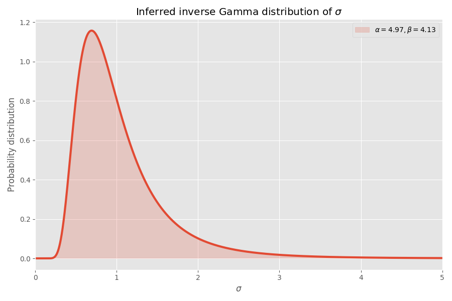
Note that values like σ > 4 are incredibly unlikely, but when they happen, they cause a mean blowup of several thousand times.
Why software tasks always take longer than you think
Assuming this dataset is representative of software development (questionable!), we can infer some more numbers. We have the parameters for the t-distribution, so we can compute the mean time it takes to complete a task, without knowing the σ for that task is.
While the median blowup factor imputed from this fit is 1x (as before), the 99% percentile blowup factor is 32x, but if you go to 99.99% percentile, it’s a whopping 55 million! One (hand wavy) interpretation is that some tasks end up being essentially impossible to do. In fact, these extreme edge cases have such an outsize impact on the mean, that the mean blowup factor of any task ends up being infinite. This is pretty bad news for people trying to hit deadlines!
Summary
If my model is right (a big if) then here’s what we can learn:
- People estimate the median completion time well, but not the mean.
- The mean turns out to be substantially worse than the median, due to the distribution being skewed (log-normally).
- When you add up the estimates for n tasks, things get even worse.
- Tasks with the most uncertainty (rather the biggest size) can often dominate the mean time it takes to complete all tasks.
- The mean time to complete a task we know nothing about is actually infinite.
Notes
- This is obviously just based on one dataset I found online. Other datasets may give different results.
- My model is of course also highly subjective, like any statistical model.
- I would ❤️ to apply the model to a much larger data set to see how well it holds up.
- I assumed all tasks independent. In reality they might have a correlation which would make the analysis a lot more annoying but (I think) ultimately with similar conclusions.
- The sum of log-normally distributed value is not another log-normally distributed value. This is a weakness with that distribution, since you could argue most tasks is really just a sum of sub-tasks and it would be nice if our distribution was stable like that.
- I removed small tasks (estimated time less than or equal to 7 hours) from the histogram since small tasks skew the analysis and there there was an odd spike at exactly 7.
- The code is on my Github, as usual.
- There’s some discussion on Hacker News and on Reddit.